Entering the Pivot Table Data

The first step in creating a pivot table is to enter the data into the worksheet.

When doing so, keep the following points in mind:

• At least three columns of data are needed to create a pivot table.
• It is important to enter data correctly. Errors, caused by incorrect data entry, are the source of many problems related to data management.
• Leave no blank rows or columns when entering the data. This includes NOT leaving a blank row between the column headings and the first row of data.

 

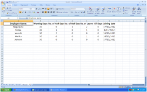
Enter the data into cells A1 to G6 as seen in the image above. 

Creating the Pivot Table

1. Drag select cells A2 to G6  to highlight them.
2. Click on the Insert tab of the ribbon.
3. Click on the down arrow at the bottom of Pivot Table button to open the drop down list.
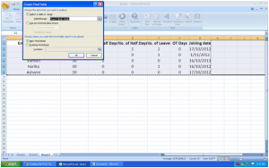
4. Click on Pivot Table in the list to open the Create Pivot Table dialog box.
5. By pre-selecting the data range A2 to G6,the Table/Range line in the dialog box should be filled in for us.
6. Choose New Worksheet for the location of the pivot table.

7. Click OK.

 

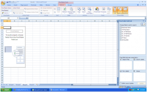
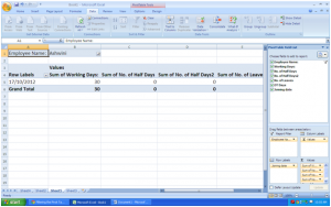
A blank pivot table should appear on the new  worksheet as shown in the above image.

 

The Pivot Table Field List panel should open on the right hand side of the Excel window.

At the top of the Pivot Table Field List panel are the field names ( column headings ) from our data table. The data areas at the bottom of the panel are linked to the pivot table.

 

Adding Data to the Pivot Table

You have two choices when it comes to adding data to the Pivot Table:

• Drag the field names from the Pivot Table Field List panel and drop them on the Pivot Table in the worksheet.
• Drag the field names to the bottom of the Pivot Table Field List panel and drop them in the data areas.

 

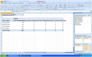
The data areas in the Pivot Table Field List panel are linked to corresponding areas of the pivot table. As you add the field names to the data areas, your data is added to the pivot table.

Depending on which fields are placed in which data area, different results can be obtained.

Filtering the Pivot Table Data

The Pivot Table has built in filtering tools that can be used to fine tune the results shown by the Pivot Table.

Filtering data involves using specific criteria to limit what data is displayed by the Pivot Table.

1. Click on the down arrow next to the All  heading in the Pivot Table to open the filter’s drop down list.
2. Click on the check box next to the Select All option to remove the check mark from all the boxes in this list.
3. Click on the check boxes next and select the particular one options to add check marks to these boxes.
4. Click OK.
5. The Pivot Table should now show only the selected data.